Variational Autoencoder
[TOC]
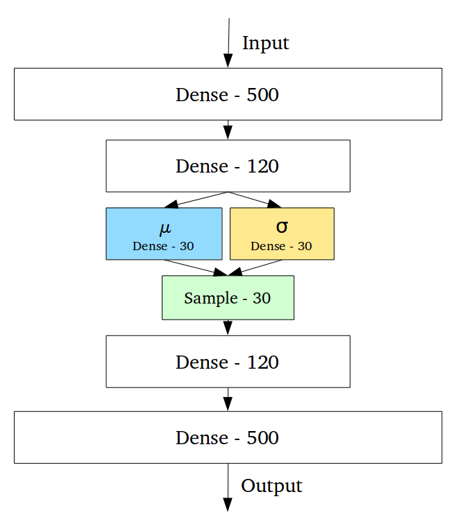
Neural Network Perspective
(This graph switches the $\theta$ and $ \phi$ comparing to the original VAE paper.)

The model:
- Generative Model $ p_{\theta}(z)p_{\theta}(x|z) $.
- Variational Approximation $ q_{\phi}(z|x) $ to the intractable posterior $ p_{\theta}(z|x) $.
Difference from Vanilla Autoencoder
"The fundamental problem with autoencoders is that the latent space may not be continuous.
Variational Autoencoders (VAEs) have one fundamentally unique property that separates them from vanilla autoencoders (and it is this property that makes them so useful for generative modeling): their latent spaces are by design continuous, allowing easy random sampling and interpolation."
-- Intuitively Understanding Variational Autoencoders
Problem (📄)
Scenario:
Dataset $ X = \{ x^{(i)} \}_{i=1}^{N}$ is generated by some random process which involves an unobserved continuous random variable $ z $. The process of generation:
- A $ z^{(i)} $ is generated from some prior distribution $ p_{\theta^{*}}(z) $, which comes from a parametric family of distribution $ p_{\theta}(z) $.
- An $ x^{(i)} $ is generated from some conditional distribution $ p_{\theta^{*}}(x|z) $, which comes from a parametric family of distribution $ p_{\theta}(x|z) $.
Our Interests:
We want a general algorithm that works efficiently in case of:
- Intractability: The marginal likelihood $ p_{\theta}(x) = \int p_{\theta}(z)p_{\theta}(x|z) dz $ is intractable, so is the true posterior density $ p_{\theta}(z|x) = \frac{p_{\theta}(x|z)p_{\theta}(z)}{p_{\theta}(x)} $.
- A large dataset.
So we propose a solution to three related problems in the above scenario:
- Efficient approximate MLE or MAP estimation for the parameter $ \theta $.
- Efficient approximate posterior inference of the latent variable $ z $ given an observed value $ x $ for a choice of $ \theta $.
- Efficient approximate marginal inference of the variable $ x $.
Solution:
We introduce a recognition model $ q_{\phi}(z|x) $: an approximation to the intractable true posterior $ p_\theta(z|x) $. We introduce a method for learning the recognition model parameters $ \phi $ jointly with the generative model parameters $ \theta $.
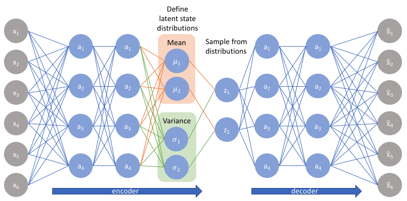
- We refer to the recognition model $ q_\phi(z|x) $ as a probabilistic encoder, since given a datapoint $ x $ it produces a distribution over the possible values of the code $ z $ from which the datapoint $ x $ could have been generated.
- In a similar vein we will refer to $ p_\theta(x|z) $ as a probabilistic decoder, since given a code $ z $ it produces a distribution over the possible corresponding values of $ x $.
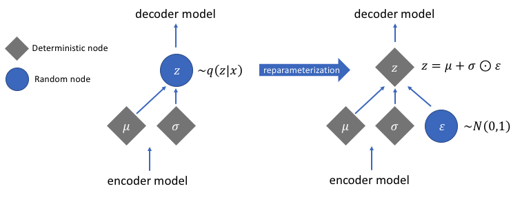
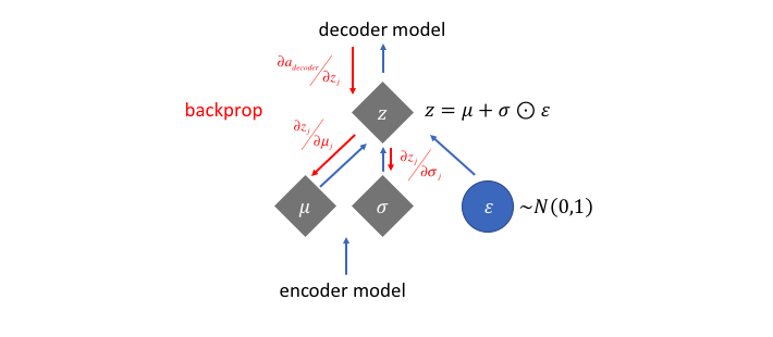
Trick:
Convert probability distribution $ z \sim p_\phi(z|x) $ to a deterministic function $ \underline{z} = g_\phi(\underline{x}, \underline{\epsilon}) $ where $ \underline{\epsilon} $ is a noise random variable. For example, $ g_\phi(\underline{x}, \underline{\epsilon}) = \underline{\mu} + \underline{\sigma} \odot \underline{\epsilon} $.
Objective
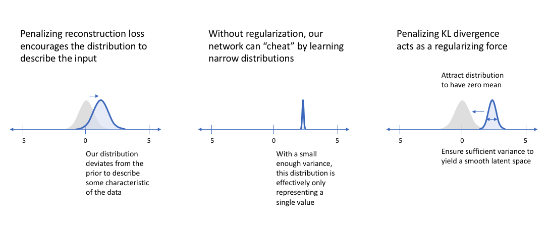
$$ \begin{aligned} D_{KL}(q_\phi \Vert p_\theta) &= \mathbb{E}_{q_\phi} \left[\log \frac{1}{p_\theta} - \log \frac{1}{q_\phi} \right] = \mathbb{E}_{q_\phi} \left[ \log q_\phi - \log p_\theta \right] \\ \ell(\theta, \phi; x_i, z) &= \mathbb{E}_{z \sim q_\phi(z|x_i)} \left[ \log \frac{1}{p_{\theta}(x_i|z)} \right] + D_{KL}(q_\phi(z|x_i) \Vert p(z)) \\ &= \ell_{\text{Reconstruction}} + \ell_{\text{Distribution}} \\ \mathcal{L}(\theta, \phi; x, z) &= \sum_{i=1}^{N} \ell_i \end{aligned} $$For reconstruction loss. $$ \begin{aligned} \mathbb{E}_{z \sim q_\phi(z|x_i)} \left[ \log \frac{1}{p_{\theta}(x_i|z)} \right] \end{aligned} $$ If the $ z $ that encodes $ xi $ and the decoder is good, then $ p\theta(x_i|z) $ is large, which means the reconstruction loss is small. So this term encourages the decoder to reconstruct the data well.
For distribution loss: $$ D_{KL}(q_\phi(z|x_i) \Vert p(z)) $$ In the variational autoencoder, $ p(z) $ is specified as $ \mathcal{N}(0, 1) $. This term encourages the encoder the keep the representation of each digit sufficiently diverse.
If we did not include this term, then the encoder could learn to cheat by giving each datapoint a representation in a different region of Euclidian space(e.g. $2_{a}$ and $2_b$ could have completely different representation $z_{a}$ and $z_b$) so as to mimic the data. This term keeps similar numbers’ representations close together. Hence we need our prior $ p(z) $.
Loss Function - ELBO View (📄)
$$ \begin{aligned} \log p(x) &= \mathbb{E}_{z \sim q_\phi(z|x)}\left[\log p(x)\right] \\ &= \mathbb{E}_{z \sim q_\phi(z|x)}\left[\log \frac{p(x|z)p(z)}{p(z|x)} \right] \\ &= \mathbb{E}_{z \sim q_\phi(z|x)}\left[\log \frac{p(x|z)p(z)}{p(z|x)} \frac{q_\phi(z|x)}{q_\phi(z|x)} \right] \\ &= \mathbb{E}_{z \sim q_\phi(z|x)}\left[\log p(x|z) + \log \frac{p(z)}{q_\phi(z|x)} + \log\frac{q_\phi(z|x)}{p(z|x)} \right] \\ &= \mathbb{E}_{z \sim q_\phi(z|x)}\left[\log p(x|z) - \log \frac{q_\phi(z|x)}{p(z)} + \log\frac{q_\phi(z|x)}{p(z|x)} \right] \\ &= \mathbb{E}_{z \sim q_\phi(z|x)}\left[\log p(x|z) \right] - D_{KL}(q_\phi(z|x) \Vert p(z)) + D_{KL}(q_\phi(z|x) \Vert p(z|x)) \\ &= \left[ \mathbb{E}_{z \sim q_\phi(z|x)}\left[\log p(x|z) \right] - D_{KL}(q_\phi(z|x) \Vert p(z)) \right] + D_{KL}(q_\phi(z|x) \Vert p(z|x)) \\ &= \left[ \mathbb{E}_{z \sim q_\phi(z|x)}\left[\log p_\theta(x|z) \right] - D_{KL}(q_\phi(z|x) \Vert p(z)) \right] + D_{KL}(q_\phi(z|x) \Vert p(z|x)) \\ \end{aligned} $$Since $ p(z|x) $ is intractable, we have no idea how to approach the last term. However, we know it is $ \geq 0$. The first two terms constitutes a tractable lower bound for the data probability, called ELBO. Given $ x $, we want to maximize the lower bound.
Loss Function - Intuitive View (👍)
Our goal: $$ \begin{aligned} q_{\phi}^{*}(z|x) &= \arg \min_{\phi} D_{KL}(q_{\phi}(z|x) \Vert p(z|x)) \end{aligned} $$
But $ p(x|z) $ is intractable. Therefore:
$$ \begin{aligned} D_{KL}(q_\phi(z|x) \Vert p(z|x)) &= \mathbb{E}_{z \sim q_\phi(z|x)} \left[\log \frac{q_\phi(z|x)}{p(z|x)} \right] \\ &= \mathbb{E}_{z \sim q_\phi(z|x)} \left[ \log \frac{q_\phi(z|x)}{\frac{p(x|z)p(z)}{p(x)}} \right] \\ &= \mathbb{E}_{z \sim q_\phi(z|x)} \left[ \log \frac{q_\phi(z|x)}{p(z)} \frac{p(x)}{p(x|z)} \right] \\ &= \mathbb{E}_{z \sim q_\phi(z|x)} \left[ \log \frac{q_\phi(z|x)}{p(z)} \right] + \mathbb{E}_{z \sim q_\phi(z|x)} \left[ \log p(x) \right] - \mathbb{E}_{z \sim q_\phi(z|x)} \left[ \log p(x|z) \right] \\ &= D_{KL}(q_\phi(z|x) \Vert p(z)) + \mathbb{E}_{z \sim q_\phi(z|x)} \left[ \log p(x) \right] - \mathbb{E}_{z \sim q_\phi(z|x)} \left[ \log p(x|z) \right] \\ &= \left[ D_{KL}(q_\phi(z|x) \Vert p(z)) - \mathbb{E}_{z \sim q_\phi(z|x)} \left[ \log p(x|z) \right] \right] + \log p(x) \\ \min_{\phi} D_{KL}(q_\phi(z|x) \Vert p(z|x)) &= \min_{\phi} \left[ D_{KL}(q_\phi(z|x) \Vert p(z)) - \mathbb{E}_{z \sim q_\phi(z|x)} \left[ \log p(x|z) \right] \right] \\ &= \min_{\phi, \theta} \left[ D_{KL}(q_\phi(z|x) \Vert p(z)) - \mathbb{E}_{z \sim q_\phi(z|x)} \left[ \log p_{\theta}(x|z) \right] \right] \\ \end{aligned} $$How to Train
Originally the loss cannot backpropagates through the sampling/stochastic part. The internal representation we learn are statistical properties for continuous variables! Reparameterization trick is used to consolidate a formula for the sampled latent vector with $\epsilon$, so that backpropagation can be used. The network is split up into a part where we can do backpropagation and a part that is stochastic yet we do not need to train.
Algebra / Term
- $ q_\phi(\underline{z} | \underline{x})$: The representation of a neural network. / Represents a distribution since it also serves as a pdf function. / The encoder.
- $ p_\theta(\underline{x} | \underline{z}) $: The representation of another neural network. / Represents a distribution since it is a pdf function. / The decoder.